
Rey.BEng prompt, authored by Grok 19/8/26
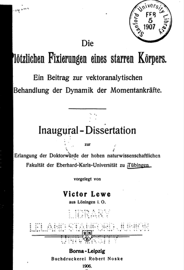
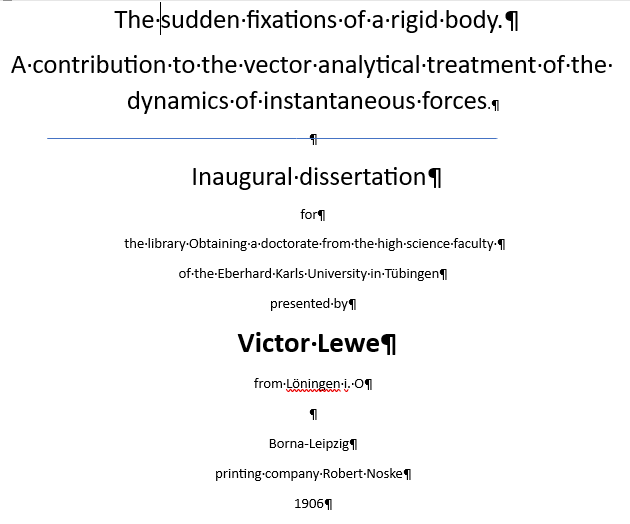
Accepted by the Faculty on 31 May 1906.
Rey.BEng and Grok, 24th August 2026 – A clear walk-through of Lewe 1906 – Sudden Fixations of a Rigid Body (for curious minds)
Imagine a free rigid body flying through space, spinning and translating. Suddenly you grab one of its points and hold that point still. What happens to the rest of the body?
That is the central question Lewe answers.
1. Impulsive forces
An ordinary force that acts for a very short time can still deliver a finite “kick.” The kick is called an impulse. It changes velocities instantly but does not have time to move anything, so positions stay the same at the moment of the kick.
2. Two global rules
After any set of impulses the body must still obey two simple balance laws:
- The total linear momentum of the centre of mass changes by exactly the sum of the external impulses.
- The total angular momentum about any fixed point changes by exactly the sum of the moments of those impulses.
3. Fixing one point
When you suddenly freeze a single point O, the only motion left is pure rotation about some axis through O.
Lewe writes the angular-momentum balance about O and solves for the new angular-velocity vector.
If the axes are chosen as the principal axes of inertia at O, the three components separate and the answer is immediate.4. Fixing a straight line (or two points)
The body is now forced to rotate about that line.
The component of angular momentum along the line cannot be changed by the impulsive reactions (they have no moment about the line).
Therefore the new spin about the line is simply (old angular momentum along the line) ÷ (moment of inertia about the line).
5. The clever reduction
What if the point is not brought to rest but is given some new non-zero velocity?
Lewe’s trick: invent a moving frame that already has exactly that new velocity.
In the moving frame the point is at rest, so the problem reduces to an ordinary fixation.
He proves (with a short vector argument) that the angular-momentum balance keeps the same form in the moving frame (Coriolis’ theorem). Solve the fixation relative to the moving frame, then transform back to the laboratory. Done.
6. The impulsive reactions
Once the new motion is known, the two global balance laws immediately give the total impulsive force and the total impulsive moment that the supports must have exerted.
7. Kinetic energy
The same balance laws also deliver the classical energy theorems (Thomson–Tait, Carnot, Appell) in a few lines of vector algebra: the loss of kinetic energy equals the kinetic energy of the relative motion that the constraint destroys.That is the whole logical chain.
Lewe’s contribution is not a new physical principle but a transparent, vector-based method that makes every step visible and reduces the general case to the simplest fixation problems.
This is the accurate content of the 1906 dissertation, presented so that a bright first-year student can follow it without difficulty.
To Lewe;
Introduction
Beside the finite forces, impulsive forces play a role in the dynamics of the rigid body. In the impact of rigid bodies, forces of very great intensity and very short duration appear. They produce a sudden change of velocity without change of position. The time-integral of the force, taken over the duration of the impact, is the impulsive force.
In the dynamics of impulsive forces the problems to be solved fall into two kinds, according as the sudden change of the state of motion is to be calculated from given impulsive forces or from given constraints that individual points of the system of rigid bodies under consideration must satisfy. As long as the sudden constraints consist in prescribing the paths (the trajectories) of individual points of the system, the application of the Lagrangian equations transformed for impulsive forces always leads to the goal. Those equations cannot, however, be applied in general when individual points of the system are suddenly prescribed or forced to take new velocities. This kind of constraint is treated in the following investigation for the case of a single rigid body, with preferential use of vector-analytical methods.
In problems of this kind the questions to be answered are: the new state of motion of the body, the impulsive forces that appear, and the change in the kinetic energy.
The first question is treated in Routh’s Dynamics, §§ 288 ff., under the designation “sudden fixations.” The use of vector analysis compelled a different manner of treatment and a precisely reversed reduction of the more difficult problems to simpler ones. This required the use of Coriolis’ theorem on relative motion. It is proved here, with the aid of vector analysis, in a form that is probably new and simple.
In answering the second question the theory of centrifugal forces is also touched upon; their resultant appears in a remarkably clear form when written vector-analytically.
The answer to the third question is given by certain theorems, some of them already known, whose proof is here given for the first time in vector-analytical form. For this purpose an expression for the kinetic energy is set up and used that has the peculiarity of depending in its outward form on an arbitrarily chosen reference point in the body. The characteristic feature of this manner of proof lies in its brevity, which reveals the inner nature of the transformations in a way that could hardly be achieved without the use of vector analysis. The latter is shown by a comparison between the proof given here and the usual proofs of the theorem of Thomson and Tait (Natural Philosophy, Part I, § 309), of Carnot’s theorem, and of a theorem of Appell (Mécanique rationnelle, tome II, p. 498). In addition, a generalisation of the theorem of Thomson and Tait is proved, and by means of this and of Appell’s theorem a further theorem is established that gives for the kinetic energy of the relative motion a decomposition similar to that which the generalised Thomson–Tait theorem gives for the change of kinetic energy.
Remarks on notation
Vector-analytical rules and operational symbols are chosen in agreement with the textbooks of R. Gans, Vektoranalysis, and Abraham & Föppl, Theorie der Elektrizität I.
For the sake of brevity the meaning of the symbols occurring in the treatise is stated once and for all in advance.
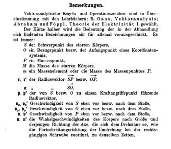
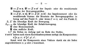
Symbol table for the 1906 translation
(We will use these consistently throughout. They stay faithful to Lewe’s meanings while being easy to type and copy-paste.)
| Lewe’s concept | Symbol we will use | Notes |
|---|---|---|
| Centre of mass | S | — |
| Arbitrary reference point | O | — |
| A general mass point | P | — |
| Total mass of the body | M | — |
| Mass of a mass element | m | — |
| Position vector from S to P | r | — |
| Position vector from O to P | r’ | — |
| Vector from S to O | a | a = SO |
| Position vector from S (or O) to a force point | p or p’ | — |
| Velocity of S before the impulse | vS | — |
| Velocity of S after the impulse | vS’ | — |
| Velocity of O before / after | vO / vO’ | — |
| Velocity of point P before / after | v / v’ | — |
| Angular-velocity vector before | ω | (Lewe’s u) |
| Angular-velocity vector after | ω’ | (Lewe’s u’) |
| Linear momentum (Σ m v) | B / B’ | before / after |
| Angular momentum about O | U / U’ | before / after |
| Kinetic energy | T / T’ | before / after (Lewe’s L) |
| Kinetic energy of the relative motion | T_rel | — |
| Impulsive force | G | — |
| Ordinary (finite) force | F | (Lewe’s P) |
| Time at beginning / end of impulse | t / t’ | — |
Tricky or vector-product notation:
- Vector cross product will be written [A × B]
- Scalar product will be written A · B
§ 1. The impulsive forces, the centre-of-mass theorem and the angular-momentum theorem applied to them
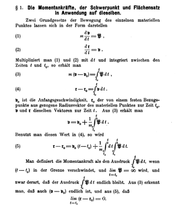
Two fundamental laws of the motion of a single material point can be written in the form
(1) m dv/dt = F
(2) dr/dt = v
If one multiplies (1) and (2) by dt and integrates between the times t and t₀, one obtains
(3) m (v – v₀) = ∫_{t₀}^t F dt
(4) r – r₀ = ∫_{t₀}^t v dt
Here v₀ is the initial velocity, r₀ the radius vector of the material point drawn from a fixed reference point at time t₀; v and r are the same vectors at time t. From (3) one has
v = v₀ + (1/m) ∫_{t₀}^t F dt
Substitution of this value into (4) yields
(5) r – r₀ = v₀ (t – t₀) + (1/m) ∫_{t₀}^t ∫ F dt dt
One defines the impulsive force as the expression ∫_{t₀}^t F dt when (t – t₀) tends to the limit zero and lim F = ∞, in such a way that the integral remains finite. From (3) one sees that (v – v₀) is also finite, and from (5) that
lim (r – r₀) = 0
The impulsive force therefore produces only a change of velocity, not a change of position.
If the word “sudden” is taken to mean that a change occurs in an infinitely short time, one may also reverse the statement:
A sudden finite change of velocity can be produced only by an impulsive force.
This follows from equation (3) and the definition of the impulsive force.
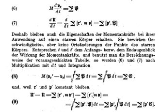
With the aid of d’Alembert’s principle one derives from equations (1) and (2) the equations of motion of the rigid body, in particular the centre-of-mass theorem and the angular-momentum theorem:
(6) M dvS / dt = Σ F
(7) dU / dt = d/dt Σ [r’ × m v] = Σ [p’ × F]
Consequently the properties of impulsive forces remain valid when they act on a rigid body. They produce changes of velocity but no changes of position of the points of the rigid body. If t and t’ correspond to the beginning and the end of the action of the impulsive forces, and if the notation of the preliminary table is used, then after multiplication by dt and integration equations (6) and (7) become
(8) M (vS’ – vS) = ∫_t^{t’} Σ F dt = Σ G
and, because r’ and p’ remain constant,
(9) U’ – U = Σ [r’ × m v’] – Σ [r’ × m v] = Σ [p’ × G]
Equations (8) and (9) are the centre-of-mass theorem and the angular-momentum theorem in the dynamics of impulsive forces. They hold first for a fixed reference system and then also for a moving one; for, since impulsive forces produce no changes of position, the moving system may always be regarded as fixed at the instant under consideration. Because the integral of a finite force F over the infinitely close limits t and t’ vanishes, the action of finite forces may be neglected beside that of the impulsive forces.
The equations 1-9 are drawn by Lewe thus;
.
§ 2. The velocities that appear after the sudden fixation
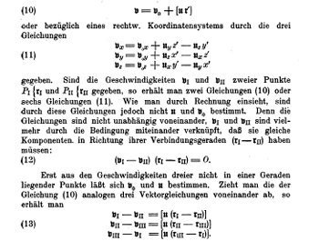
After these introductory remarks we turn to the treatment of the theme itself. The state of motion of a rigid body is given by the (translational) velocity of one of its points O and by the angular velocity about an axis through that point. The velocity of any other point P of the rigid body is then given by the vector equation
(10) v = vO + [ω × r’]
or, referred to a rectangular coordinate system, by the three equations
(11) vx = vOx + ωy z’ – ωz y’
vy = vOy + ωz x’ – ωx z’
vz = vOz + ωx y’ – ωy x’
If the velocities vI and vII of two points PI and PII are given, one obtains two equations of the form (10) or six equations of the form (11). As calculation shows, these equations do not determine ω and vO. The equations are not independent of one another; vI and vII are linked by the condition that they must have equal components in the direction of the line joining them (rI – rII):
(12) (vI – vII) · (rI – rII) = 0
Only from the velocities of three points that do not lie on a straight line can vO and ω be determined. Subtracting the three vector equations analogous to (10) from one another yields
(13) vI – vII = [ω × (rI – rII)]
vII – vIII = [ω × (rII – rIII)]
vIII – vI = [ω × (rIII – rI)]
These equations, or their nine component equations, are sufficient to determine ω and then, from one of the original equations, vO.
It is therefore clear that if more than two points that do not lie on a straight line are suddenly given new velocities that satisfy the condition (12) in pairs, the state of motion of the rigid body is thereby fixed. There remains only the case in which one or two points, or a straight line, of the free rigid body suddenly receive a new state of motion. The simplest case, in which this new state of motion consists in absolute rest, will be examined first. This problem is also called the problem of sudden fixation.
Sudden fixation of a point in the rigid body
The question to be answered first is the following:
A rigid body has the state of motion (vS, ω). Suddenly a point O of the body is fixed. What is the state of motion after the change?
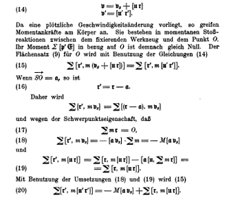
The new state of motion consists only in an angular velocity ω’ about an axis through O. The velocity v of an arbitrary point of the rigid body is, according to (10), before and after the change
(14) v = vS + [ω × r]
v’ = [ω’ × r’]
Since a sudden change of velocity is present, impulsive forces act on the body. They consist in instantaneous impact reactions between the fixing tool and the point O. Their moment about O is therefore zero. The angular-momentum theorem (9) written for the point O, with the use of equations (14), becomes
(15) Σ [r’ × m (vS + [ω × r])] = Σ [r’ × m [ω’ × r’]]
If a = SO, then
(16) r’ = r – a
Hence
Σ [r’ × m vS] = Σ [(r – a) × m vS]
and, because of the centre-of-mass property
(17) Σ m r = 0,
(18) Σ [r’ × m vS] = – M [a × vS]
and
(19) Σ [r’ × m [ω × r]] = Σ [r × m [ω × r]]
With the substitutions (18) and (19), equation (15) becomes
(20) Σ [r’ × m [ω’ × r’]] = – M [a × vS] + Σ [r × m [ω × r]]
Continuation of § 2 – Determination of the new angular velocity after fixation of a point
In order to extract the vector ω’ from the left-hand side of equation (20), one must resolve the expression into components along the axes of a rectangular coordinate system. By the vector identity
(21) [A × [B × C]] = B (A · C) – C (A · B)
one has
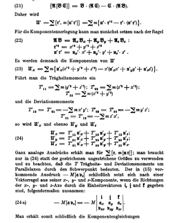
Σ [r’ × m [ω’ × r’]] = Σ m { ω’ (r’ · r’) – r’ (ω’ · r’) }
For the component resolution one first uses the rule
(22) A · B = Ax Bx + Ay By + Az Bz
so that
r’ · r’ = x’² + y’² + z’²
ω’ · r’ = ω’x x’ + ω’y y’ + ω’z z’
The x-component of the left-hand side therefore becomes
(23) Σ m { ω’x (x’² + y’² + z’²) – x’ (ω’x x’ + ω’y y’ + ω’z z’) }
Introducing the moments of inertia
T11 = Σ m (y’² + z’²), T22 = Σ m (z’² + x’²), T33 = Σ m (x’² + y’²)
and the products of inertia
T12 = T21 = – Σ m x’ y’, T23 = T32 = – Σ m y’ z’, T31 = T13 = – Σ m z’ x’
one obtains for the three components
(24) T11 ω’x + T12 ω’y + T13 ω’z = right-hand side x-component
T21 ω’x + T22 ω’y + T23 ω’z = right-hand side y-component
T31 ω’x + T32 ω’y + T33 ω’z = right-hand side z-component
Exactly analogous expressions are obtained for Σ [r × m [ω × r]]; one need only replace the primed quantities by the corresponding unprimed ones (moments and products of inertia about parallel axes through the centre of mass).
The remaining term –M [a × vS] on the right-hand side of (20) has the components given by the determinant form
(24a) –M [a × vS] = –M | i j k |
| ax ay az |
| vSx vSy vSz |
Collecting everything yields the three scalar equations
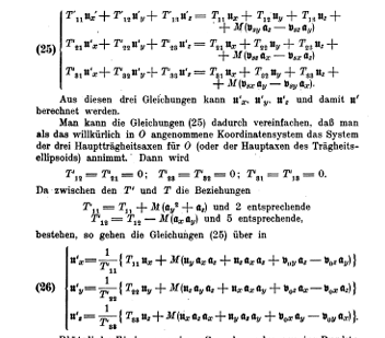
(25) T’11 ω’x + T’12 ω’y + T’13 ω’z = T11 ωx + T12 ωy + T13 ωz + M (vSy az – vSz ay)
T’21 ω’x + T’22 ω’y + T’23 ω’z = T21 ωx + T22 ωy + T23 ωz + M (vSz ax – vSx az)
T’31 ω’x + T’32 ω’y + T’33 ω’z = T31 ωx + T32 ωy + T33 ωz + M (vSx ay – vSy ax)
From these three equations the components of ω’ can be calculated.
The equations can be simplified by choosing as the coordinate system at O the principal axes of inertia at O. Then all products of inertia vanish (T’12 = T’23 = T’31 = 0) and the three equations decouple:
(26) ω’x = (1/T’11) { T11 ωx + M (terms involving a and vS) }
ω’y = (1/T’22) { T22 ωy + M (terms involving a and vS) }
ω’z = (1/T’33) { T33 ωz + M (terms involving a and vS) }
(The precise expanded form of the terms in braces is the one given by Lewe in the original.)
This determines the new angular velocity after a single point has been suddenly fixed.
Sudden fixation of a straight line or of two points in the rigid body
In the case of the sudden fixation of a straight line, or of two points, of the rigid body the impulsive forces that appear act at points of the suddenly fixed line or at the two suddenly fixed points. Their moment about this line (or about the line joining the two points) is zero. In vector language the moment about a line is defined as the scalar product of the unit vector of that line and the moment taken with respect to any point on the line.
After the fixation the body is compelled to rotate about the fixed line. The unit vector of the line is therefore the direction of the new angular-velocity vector ω’, and one has
(27) ω’₁ · Σ [p’ × G] = 0
where Σ [p’ × G] is the resultant moment about a point O on the fixed line and ω’₁ is the unit vector in the direction of ω’.
Multiplying both sides of the angular-momentum equation (9) by ω’₁ and taking account of (27) yields
(28) ω’₁ · (U’ – U) = 0
Because the velocities before and after the impulse may still be written in the form (14), equation (28) is analogous to the equation obtained by taking the scalar product of (15) or (20) with ω’₁:
(29) ω’₁ · Σ [r’ × m [ω’ × r’]] = – M ω’₁ · [a × vS] + ω’₁ · Σ [r × m [ω × r]]
The left-hand side admits a simple interpretation. By the vector identity (21)
[r’ × m [ω’ × r’]] = m (ω’ (r’ · r’) – r’ (ω’ · r’))
and therefore
ω’₁ · [r’ × m [ω’ × r’]] = m |ω’| (r’ · r’) sin²(θ)
where θ is the angle between ω’ and r’. Summing over all mass elements gives
(30) ω’₁ · Σ [r’ × m [ω’ × r’]] = |ω’| · Θ
Here Θ = Σ m r’² sin²(θ) is precisely the moment of inertia of the body about the fixed line.
Equation (29) therefore reduces to
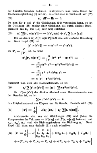
(31) |ω’| = (1/Θ) { – M ω’₁ · [a × vS] + ω’₁ · Σ [r × m [ω × r]] }
The components of the two vectors that appear on the right-hand side are already known from (24) and (24a). If l, m, n are the direction cosines of the unit vector ω’₁, one may also write
(32) |ω’| = (1/Θ) { – M | l m n ; ax ay az ; vSx vSy vSz |
+ l (T11 ωx + T12 ωy + T13 ωz)
+ m (T21 ωx + T22 ωy + T23 ωz)
+ n (T31 ωx + T32 ωy + T33 ωz) }
Thus the magnitude of the new angular velocity about the fixed line is determined.

This completes the direct treatment of the two elementary fixation problems (single point, and straight line / two points).
Reduction of the general problem of sudden velocity changes to the problem of sudden fixations
The “sudden fixations” constitute only a special case of the problem of the sudden change of velocity of one or two points or of a straight line. One can nevertheless reduce the treatment of the latter problem to that of the former by regarding the velocity change as a fixation of a point or of a line of a body that is performed inside a space previously attached to a moving coordinate system and moving with it. In this sense the fixation in the moving space is to be understood.
If the states of motion of the moving space and of the body are referred to the same reference point, then the state of motion forced upon the point or the line by the fixation in the moving space is the same as that of the moving space. From this the following possibility of solution results:
The procedure is therefore:
- Determine the state of motion of the rigid body relative to a suitably chosen moving frame (or relative to a coordinate system fixed in that frame).
- Apply the fixation formulae already derived — equations (25) or (31) — inside the moving frame.
- Transform the result back to the absolute (fixed) frame.
This method of solution is possible only if the angular-momentum equation (9), of which (25) and (31) are consequences, does not change its form when it is applied to the “moving space”. Whether this is the case is decided by Coriolis’ theorem on relative motion, which will now be derived in the simplest possible way.Relative motion
One considers the time rate of change of a vector M with respect to a frame fixed in space and with respect to a moving frame. If the second (coordinate) system moves parallel to the first, the components of a vector that is independent of the motion of the frame, and the components of its time rate of change, remain the same in both systems. Denoting by dM/dt the time rate of change in the first system and by d’M/dt that in the second system, one has
(33) dM/dt = d’M/dt
The radius vector r, on the other hand, is drawn once from the fixed point and once from the moving point. The geometric difference of the two is the joining line of the This reduction is legitimate only if the angular-momentum equation (9) retains the same form when it is written with respect to the moving frame. Whether that is true is decided by Coriolis’ theorem on relative motion, which is now derived in vector language.
Relative Motion (from the page numbered 12 in the original)
We now look at how a vector changes with time when it is measured in a fixed frame and when it is measured in a moving frame.
If the moving frame is only translating (not rotating) relative to the fixed frame, then any vector that does not depend on the motion of the frame, and its time derivative, have exactly the same components in both frames.
Writing dM/dt for the rate of change seen from the fixed frame and d’M/dt for the rate of change seen from the moving frame, we have
(33) dM/dt = d’M/dt
The position vector r is different: one version is drawn from the fixed origin, the other from the moving origin. The difference between them is simply the vector that joins the two origins.
When the moving frame is also rotating, an extra term appears.
Lewe derives the full relation and arrives at the angular-momentum theorem written in the moving frame:
(35) dU/dt = d’U/dt + [v₀ × B] = Σ [p × F]
If the moving frame is rotating with angular velocity ω and we let the two frames coincide at the instant we are interested in, the relation between the absolute and the relative rates of change of any vector M becomes
(36) dM/dt = d’M/dt + [ω × M]
and therefore
(37) dU/dt = d’U/dt + [ω × U]
Putting (35) and (37) together gives the angular-momentum theorem in the moving frame:
(38) d’U/dt + [ω × U] + [v₀ × B] = Σ [p × F]
Because v₀, U, B and F are all finite, the extra terms vanish when we integrate across the infinitely short duration of an impulse.
That is why the fixation formulae (25) and (31) can be used without change inside a moving frame.
Lewe then gives a short, clear proof of Coriolis’ theorem itself (equations (a), (b) and (39) in the original).
The final result is the familiar formula that relates absolute acceleration to relative acceleration plus the Coriolis and centripetal terms.
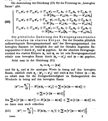
Application of the fixation formulae inside the moving frame
With the above justification, the method outlined on page 12 can now be carried out.
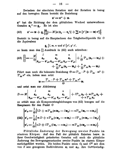
- For a single point that is suddenly given a new velocity, one simply applies equation (25) to the relative motion. This produces the three component equations numbered (40) in the original.
- For a straight line that is suddenly given the motion of the moving frame, one applies equation (31) to the relative motion. This produces equation (41) and the subsequent reductions (42)–(44).
- For two points the same idea is used, leading to equations (45)–(49).
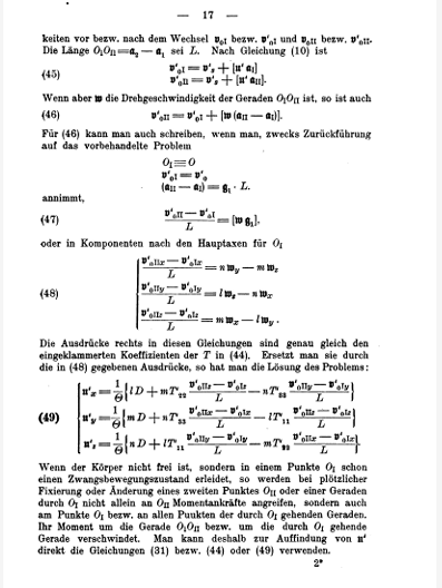
This finishes the reduction of every sudden velocity change to an ordinary fixation problem.
§ 3. The impulsive forces and impulsive force-pairs that appear at a sudden fixation or change of motion
The resultant of all the impulsive forces that appear at a sudden fixation is found at once from the centre-of-mass theorem (8):
(50) Σ G = M (vS’ – vS)
where vS’ is calculated from the known vectors vO’ (or vO’I) and ω’ by the relation
vS’ = vO’ – [ω’ × a]
(or the analogous expression for two points).
When a straight line is fixed, an impulsive force-pair also appears. It is obtained from the angular-momentum theorem (9) written about a point O (or OI) on the line:
(51) Σ [p’ × G] = – M [a × (vS’ – vS)] + Σ [r’ × m [(ω’ – ω) × r’]]
To find the two separate impulsive forces GI and GII that act at the two points OI and OII, one writes the angular-momentum theorem about each of those points together with the centre-of-mass theorem. This produces the three vector equations
(52) [(aII – aI) × GI] = – M [aI × (vS’ – vS)] + Σ [r’ × m [(ω’ – ω) × r’]]
(53) [(aI – aII) × GII] = – M [aII × (vS’ – vS)] + Σ [r’II × m [(ω’ – ω) × r’II]]
(54) GI + GII = M (vS’ – vS)
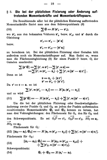
These three equations are not yet sufficient to determine GI and GII completely. One therefore resolves them in a coordinate system whose z-axis lies along the line OI OII. The components of GI and GII parallel to that line remain indeterminate; the components perpendicular to the line are uniquely determined, and their sum is already known from (54).
The resultant centrifugal force
Immediately after the impulsive forces have acted, centrifugal forces appear at the fixed point or along the fixed line.
Their resultant and their resultant moment are derived briefly.
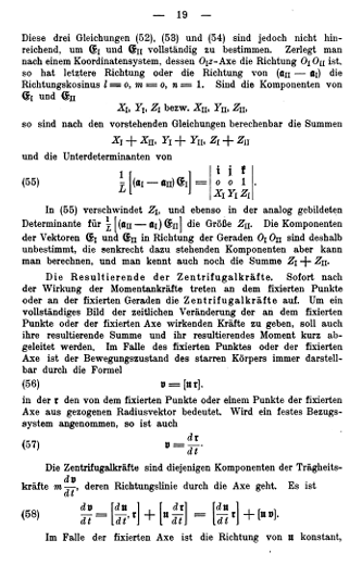
In the case of a fixed point (or fixed axis) the velocity of any point is
(56) v = [ω × r]
and therefore
(57) dv/dt = dω/dt × r + [ω × [ω × r]]
The centrifugal forces are the components of the inertial forces that are directed along the line of action of ω. Summing over the whole body yields
(59) Σ m [ω × v] = [ω × B] = M [ω × vS]
and the resultant moment of the centrifugal forces is
(60) Σ m [r × [ω × v]] = [ω × U]
Lewe states the two compact results:
Theorem 1. The resultant of the centrifugal forces is equal to the vector product of the angular velocity and the linear momentum of the body.
Theorem 2. The resultant moment of the centrifugal forces is equal to the vector product of the angular velocity and the angular momentum of the rotating body.
§ 4. The kinetic energy of the body before and after the change
The kinetic energy of a rigid body is given by the familiar expression
L = ½ Σ m v²
For the purposes of vector calculation this is rewritten
(63) 2L = vO · B + ω · U
(the form that depends on an arbitrarily chosen reference point O).
With this expression a series of theorems is derived that relate the loss of kinetic energy to the kinetic energy of the relative motion and to the impulsive forces.
The first is the theorem of Thomson and Tait.
An impulsive force G acts at a point of the body. With the notation of the table one obtains
(64) 2(L’ – L) = vO’ · B’ + ω’ · U’ – vO · B – ω · U
When the vectors are referred to the point of application of the impulse, the angular-momentum theorem and the centre-of-mass theorem simplify the right-hand side, and one arrives at
(67) L’ – L = G · ½ (vO’ + vO)
A completely analogous calculation for an impulsive force-pair yields
(72) L’ – L = K · ½ (ω’ + ω)
where K is the moment of the force-pair.
The same reasoning is then extended to the case in which several impulsive forces act at different points, giving the general statement
(74) L’ – L = Σ [G · ½ (v’ + v)]
where the sum is taken over all the points of application and v, v’ are the velocities of those points before and after the impulse.
Finally the theorems are specialised to the three elementary fixation problems (single point, straight line, two points) and to the case of a prescribed velocity change of two points.
Final part of § 4 – Kinetic energy of the relative motion, Appell’s theorem, and Carnot’s theorem
Lewe next derives a relation for the kinetic energy of the relative motion.
That energy is defined by
L_(v’–v) = ½ Σ m (v’ – v)²
With the help of the centre-of-mass and angular-momentum theorems for impulsive forces one obtains
(75) 2 L_(v’–v) = (vO’ – vO) · Σ G + (ω’ – ω) · Σ [p’ × G]
Because the velocity of the point of application of an impulse is vO + [ω × p’] (or the corresponding primed quantity), the expression simplifies at once to
(76) L_(v’–v) = Σ [ G · ½ (v’ – v) ]
where the sum runs over all points of application.
Appell’s theorem
Adding (74) and (76) yields
(77) L’ – L = – L_(v’–v) + Σ (G · v’)
In words: the sum of the products of each impulsive force with the final velocity of its point of application equals the change in the kinetic energy of the body plus the kinetic energy of the relative motion.
(This is the theorem given by Appell in Traité de mécanique rationnelle, art. 520.)
Carnot’s theorem
When two or more perfectly smooth, or perfectly rough, rigid bodies collide, the impulsive forces that act between them satisfy
Σ (G · v’) = 0
(the common points of contact have equal final velocities, or the impulses are equal and opposite).
Equation (77) therefore reduces to
(78) L’ – L = – L_(v’–v)
This is Carnot’s theorem: the loss of kinetic energy equals the kinetic energy of the relative motion that is destroyed by the impact.
The same equation (77) remains valid for a sudden absolute fixation (because the final velocities of the fixed points are zero) and therefore recovers Carnot’s theorem in that special case as well.
For a prescribed non-zero velocity change of one or two points, or of a line, the more general relation (77) takes the place of Carnot’s theorem.
With these results the dissertation ends.

