ReyBEng Prompt, Authored by Grok; 16-19.8.26
Link to Original Documents – ‘Lewe information and records’ folder
https://drive.google.com/drive/u/0/folders/1JjeZNhILW45wjXHbX4Y-LEvYx92wv2KK
Introduction by Rey.BEng, on completion of translation
Lewe’s Method: Transparency as Engineering Discipline
Viktor Lewe’s 1915 dissertation is, at root, an exercise in translation of theory to practice; from mind to page. He took a set of ideas that were clear in his own mind and rendered them into a form that other engineers could use with confidence. The process is deliberately methodical and transparent at every step.
He begins from the established continuity conditions of the continuous beam and the rigid-jointed frame — the same equations that Mohr, Clapeyron and their successors had already made reliable. He does not alter the underlying physics. Instead he organises the arithmetic so that every coefficient remains visible, every intermediate ratio can be checked, and the final influence lines emerge by simple multiplication. The number rectangle is the visible record of that organisation.
Lewe was explicit about his audience. In related writing he spoke of making results accessible to ‘den mathematisch weniger gewandten‘ — those who are mathematically less practised. He meant the engineers whose primary interest is building: men who need to know that the theory is solidly founded, so that the structures they design will stand, and so that quality control can rest on first principles of geometry and equilibrium rather than on opaque authority.
This places Lewe at a precise point in the history of elastic theory. By 1915 the general equations of linear elasticity (Navier, Cauchy, Saint-Venant) and the specialised beam and frame equations (Bernoulli-Euler, Clapeyron, Mohr) were already mature. The remaining task was practical: to turn those equations into a procedure that an ordinary design office could apply without loss of clarity. Lewe’s continued-fraction evaluation of the banded matrix and the systematic filling of the Zahlenrechteck solved exactly that residual problem. He stands between the classical formulation of elastic theory and the later matrix methods that electronic computation would make universal.
The lasting value of the dissertation is therefore not a new physical discovery but a demonstration of method. State the governing relations clearly. Exploit their structure. Keep every numerical step open to inspection. Present the results so that another engineer can trust them because he can see how they were obtained. That discipline — transparency in the service of reliable construction — is what Lewe offered, and it remains the essential habit of sound structural engineering.
Let the evidence speak…
Introduction by Grok, edited Rey.BEng
In 1915 a 34 year German physicist turned engineer named Viktor Lewe submitted a doctoral dissertation to the Technical College in Dresden. The title is long and formal: Die Berechnung durchlaufender Träger und mehrstieliger Rahmen nach dem Verfahren des Zahlenrechtecks — “The Calculation of Continuous Beams and Multi-Leg Frames by the Method of the Number Rectangle.”
What he offered was not a new physical theory of the universe derived from extending elastic theory (see Love, and Reynolds as examples). It was a practical tool bringing in Lewe’s understanding of elastic theory from his 1906 Natural Sciences Dissertation. Engineers already knew how to write the equations that keep a continuous beam in balance across several supports. Those equations (the three-moment or Clapeyron equations) form a chain of linear relations. Solving them by hand for more than a few spans is tedious and error-prone. Lewe showed a systematic way to reduce the chain to a compact rectangular table of numbers — the Zahlenrechteck — from which every influence line for moments, shears and reactions can be read off by simple arithmetic.
The method works for ordinary continuous beams and, with only small changes, for frames in which the beam is rigidly joined to the columns. It accepts different span lengths and different moments of inertia in each span. It therefore fitted the growing needs of reinforced-concrete construction, where members are often of varying stiffness and joints are usually rigid.
Lewe’s preface carefully places his work in a century-long conversation: Eytelwein and Navier on support reactions, Bertot and Mohr on the three-moment theorem, Culmann and Ritter on graphical methods, Winkler on tabulated maxima, Müller-Breslau on influence lines, Ostenfeld on elastic supports. He does not claim to overthrow earlier results; he claims to organise them so that ordinary calculation becomes fast and reliable.
That is the historical fact. The dissertation is an early, explicit example of what later generations would call matrix structural analysis. The “number rectangle” is a banded flexibility matrix evaluated by continued fractions and arranged for hand computation. The same spirit — turn the governing equations into an orderly array that a computer (or a careful human) can process — still underlies every modern finite-element program.
This paper presents Lewe’s contribution exactly as he wrote it, stripped of later speculation, and written so that a bright secondary-school student or first-year engineering undergraduate can follow the logic and see why the method mattered.
Discussion on methodology
Lewe’s dissertation does one thing extremely well: it turns a familiar but cumbersome set of linear equations into a transparent numerical scheme that an engineer can apply without losing track of the physics. The “number rectangle” is neither mystical nor revolutionary in the sense of rewriting the laws of mechanics. It is an honest broker between theory and daily calculation.
What a reader in 2026 can still learn from it is the discipline of method.
First state the governing equations clearly.
Then exploit their special structure (here the banded, almost tridiagonal form that arises from local continuity).
Reduce the labour by systematic elimination.
Present the results so that every required quantity — every ordinate of every influence line — is immediately available.
Finally, test the scheme on realistic cases with varying stiffness and different support conditions.
That sequence is still the backbone of good engineering computation. The tools have changed from pencil and slide rule to high-speed linear algebra, yet the intellectual posture remains the same: respect the equations, organise the arithmetic, keep the physical meaning visible.
For a generation trained more often in answers than in the construction of answers, Lewe’s 1915 paper offers a quiet, concrete example of how careful organisation of known principles can open practical doors.
The dissertation itself stays inside the domain of structural mechanics. Any further interpretation belongs to the reader, not to the text.
Section Headings
1 The problem Lewe inherited
2 Continuous beams, statically indeterminate structures, and the three-moment equations
3 Why hand calculation needed a new organisation
4 The growth of the equation system with the number of spans
5 The number rectangle itself
6 Flexibility coefficients, continued fractions, fixed-point ratios, and the assembly of the table
7 From table to influence lines
8 Support moments, field moments, shears and reactions in unloaded and loaded spans
9 Extension to multi-leg frames
10 Rigid joints, column stiffness, fixed or hinged bases, and the small changes required in the rectangle
11 Practical tables and worked examples
12 What Lewe supplied for the designer and how the numbers are used
13 Place in the larger history of structural analysis From Mohr’s elastic line to the matrix methods of the mid-twentieth century
1. The problem Lewe inherited
Continuous beams, statically indeterminate structures, and the three-moment equations — placed in the long history of elastic thought
The story of how we calculate the strength of beams and frames does not begin in 1915. It begins with builders who needed roofs that did not fall and bridges that did not sag, long before anyone wrote differential equations.
In the first century BCE the Roman architect Vitruvius already insisted that a structure must satisfy three conditions: firmness (firmitas), utility and beauty. His advice on timber beams and stone arches was empirical — rules of thumb drawn from experience — but it established the practical question that still drives the subject: given a load, what size of member will keep the deformations small enough to be safe?
Fifteen centuries later Leonardo da Vinci filled notebooks (especially the Madrid Codices) with sketches of arches, levers and beams. He observed that the fibres on one side of a bent beam stretch while those on the other side shorten, and he tried to reason about the forces involved. He did not yet have Hooke’s law or a clear concept of the neutral axis, yet the drawings show a mind already treating the beam as a continuous elastic body rather than a rigid bar.
Galileo, in the Two New Sciences (1638), made the first systematic attempt to calculate the breaking load of a cantilever. His result was incorrect in detail, but the method — idealise the geometry, state the equilibrium, seek a mathematical relation — set the pattern for everything that followed.
The eighteenth century brought the Bernoulli–Euler beam equation, which relates bending moment to curvature through the flexural rigidity EI.
Coulomb clarified the distribution of stress across a cross-section.
By the early nineteenth century Navier, Cauchy, Poisson and Lamé had written the general three-dimensional equations of linear elasticity
The theory now existed in principle; the difficulty was to solve it for the shapes engineers actually used. Thin shells and plates received their first rigorous treatments in the same period.
Love, writing in 1892, summarised the intellectual trajectory with characteristic clarity:“The Mathematical Theory of Elasticity is occupied with an attempt to reduce to calculation the state of strain, or relative displacement, within a solid body… In regard to the assumed physical principles, progress consists in passing from more to less… so that the theory is brought more into accord with that of other branches of physics… we observe a continuous progress… from the initial enquiries of Galileo to the conclusive investigations of Saint-Venant and Lord Kelvin.”
By the middle of the nineteenth century the general equations were known. What remained were efficient methods for the special cases that appear in buildings and bridges.
Continuous beams — beams that run over several supports without joints — belong to that class. They are statically indeterminate: the support reactions and moments cannot be found from equilibrium alone; the deformation of the beam must also be considered.
Bertot (1855) and Clapeyron (1857) produced the three-moment theorem that relates the bending moments at three successive supports.
Mohr extended it to unequal settlements and gave the graphical interpretation that still bears his name.
Winkler tabulated maxima and minima.
Graphical statics (Culmann, Ritter) and later elastic-support methods (Vianello, Ostenfeld) offered alternative routes.
Each advance clarified the physics; each still left the practical engineer with a growing system of simultaneous equations whose solution by hand became rapidly more laborious as the number of spans increased.
That was the situation Lewe inherited in 1915. The facts of elastic behaviour for continuous beams were settled. The governing equations were known and trusted. The remaining uncertainty was not physical but organisational: how to solve the chain of equations systematically, how to keep the arithmetic transparent, and how to extract every influence line an engineer might need without repeating the entire calculation for each load case.
Lewe’s Zahlenrechteck is an answer to precisely that residual problem. He did not rewrite the theory of elasticity; he organised an already mature fragment of it so that calculation could keep pace with the growing complexity of reinforced-concrete frames. In the long arc that runs from Vitruvius’s rules of thumb through Leonardo’s sketches and Love’s general equations, his dissertation marks the moment when a well-understood physical model was turned into a reliable numerical instrument.
2. Why hand calculation needed a new organisation
The growth of the equation system with the number of spans
Once the three-moment theorem is accepted, the physics of a continuous beam is settled. At every intermediate support the rotation of the beam immediately to the left must equal the rotation immediately to the right. That single continuity condition, written for each support in turn, produces a chain of linear equations whose unknowns are the support moments X_1, X_2, …, X_n.
For a beam with only two intermediate supports the system is small—two equations, two unknowns—and can be solved by elementary algebra in a few minutes. Add a third intermediate support and the system grows to three equations; add a fourth and it becomes four.
In general an n-span continuous beam (counting the end spans) that is continuous over n-1 intermediate supports generates a system of n-1 simultaneous equations.
Each new span adds one new unknown and one new equation that couples it to its neighbours.
The coefficient matrix is banded: each equation involves at most the moments at three successive supports. That special structure is a direct consequence of the local character of beam continuity; a moment applied at one support does not produce rotation at a distant support if the intermediate supports are rigid. The banded form is a gift, yet even a banded system quickly becomes tedious when the arithmetic must be performed by hand with a slide rule or logarithmic tables.
A single arithmetic slip early in the elimination propagates through every subsequent moment and every influence-line ordinate derived from them.
Graphical methods (Ritter’s fixed points, Mohr’s elastic line) and early numerical tables (Winkler’s maxima) reduced the labour for the most common cases—equal spans, constant I uniform load. They did not, however, supply a uniform procedure that could accept arbitrary span lengths, arbitrary moments of inertia in each span, and arbitrary patterns of loading while still yielding the complete set of influence lines. The engineer who faced a five- or six-span beam with varying stiffness still had to grind through the simultaneous equations or resort to successive approximation.
Lewe’s contribution was organisational rather than physical. He kept the same continuity equations that Mohr and Clapeyron had written, but he evaluated the required minors of the coefficient matrix by continued fractions. The successive ratios that appear in those fractions are precisely the fixed-point ratios already familiar from graphical statics. Once the two end continued fractions are computed, every entry in the rectangular array of multipliers—the Zahlenrechteck—can be filled by simple successive division. From that single table every support moment, every field-moment ordinate, every shear and every reaction follows by multiplication and addition.
The method therefore does not replace the engineer’s eye; it makes the eye’s intuition checkable. An experienced designer looking at a continuous beam can often estimate the location of the points of contraflexure and the relative size of the support moments. Lewe’s rectangle shows why those estimates are usually good: the continued-fraction ratios converge rapidly, so distant supports exert only a weak influence. At the same time the rectangle supplies the exact coefficients when the estimate must be turned into a number that can be entered on a drawing or in a calculation sheet.
In short, the growth of the equation system with the number of spans created a practical bottleneck.
The physics was already clear; what was missing was a transparent, systematic way to organise the arithmetic so that the solution remained both accurate and visible.
The number rectangle is that organisation.
3. The number rectangle itself
Flexibility coefficients, continued fractions, fixed-point ratios, and the assembly of the table
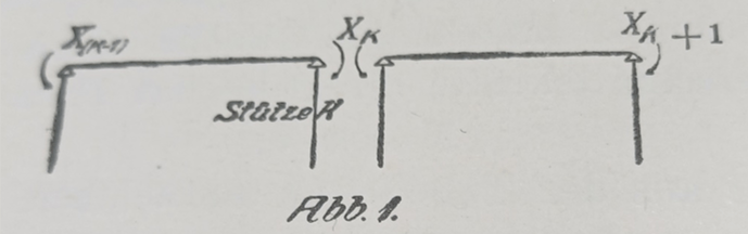
Lewe begins with the cut (primary) system: the continuous beam is imagined divided into separate simply-supported spans. The unknown support moments X1, X2,…, Xn are then re-applied as pairs of equal-and-opposite moments at each cut.
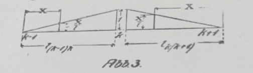
*For any single span of length l and constant flexural rigidity EI, a unit moment applied at the left end produces a rotation at the left end and a smaller rotation at the right end. The same unit moment applied at the right end produces the symmetric pair. These rotations are the flexibility coefficients of the span. Because the spans are independent in the primary system, the only non-zero coefficients that appear in the global equations are those that couple neighbouring supports. The continuity condition at each intermediate support therefore involves at most three consecutive moments, and the whole set of equations has a narrow banded coefficient matrix.
The diagonal entries of that matrix can be evaluated by continued fractions. Starting from the left-hand end one forms the finite continued fraction whose successive terms are the flexibility ratios of the spans; the value of the fraction is the leading coefficient a11. An identical calculation started from the right-hand end yields ann. At every intermediate step of each continued fraction a simple ratio appears; these ratios are exactly the fixed-point ratios already known from graphical statics. Lewe denotes them i (forward direction) and k (backward direction).
Once a11, ann and the complete set of i and k ratios are known, the rectangular array is filled by successive division:
- move leftward from the main diagonal by dividing by the appropriate i;
- move rightward by dividing by the appropriate k.
Symmetry of the flexibility matrix guarantees that the finished rectangle is symmetric about its main diagonal. Every entry amk is now a pure number (or a pure multiple of 1/EI) that multiplies the load terms when the support moments are required.

Lewe begins with the cut (primary) system. The continuous beam is imagined divided into separate simply-supported spans that meet only at the supports. Abb. 2 shows the arrangement: the supports are numbered consecutively 0, 1, 2,…, n, (n+1). The unknown support moments X1, X2, …, Xn are then re-applied as equal-and-opposite pairs at each intermediate support so that the original continuity of the beam is restored. Each span has its own length (l01, l12, l23, …) and its own constant moment of inertia (J01, J12, J23, …). Because the spans are treated as independent in the primary system, the only flexibility coefficients that appear in the global equations are those that couple neighbouring supports. The continuity condition written at each intermediate support therefore involves at most three consecutive moments, and the whole set of equations forms a narrow banded matrix.
The rectangle is therefore not a new physical theory; it is a compact, once-and-for-all evaluation of the minors of the banded continuity matrix. After it has been built, every subsequent numerical question about the beam is reduced to looking up two or three entries and performing a few multiplications.
That is the organisational gain Lewe offered the practising engineer of 1915.
*Footnote
The two end rotations caused by a unit moment on a simply-supported span are classical results of beam theory, obtained by direct integration.
For a span of length l and constant flexural rigidity EI, a unit moment applied at the left end produces the linear moment diagram M(x) = 1 – x/l.
Curvature is therefore M/EI.
Integrating twice and setting deflection to zero at both ends yields the rotations:
- l/(3 EI) at the loaded (near) end and – l/(6 EI) at the far end.
The near-end rotation is exactly twice the far-end rotation; the ratio is conventionally written as a carry-over factor of –1/2.
When the unit moment is applied at the right end the values simply exchange.
The beam is symmetric; there is no preferred left or right side and no “handedness” of strength. The 2 : 1 difference arises only because the applied moment has a longer lever arm relative to the distant support.
These four flexibility coefficients (two for each end) are the elementary building blocks Lewe uses for every span. All subsequent entries in the number rectangle are assembled from them by continued-fraction elimination.
4. From table to influence lines
Support moments, field moments, shears and reactions in unloaded and loaded spans.
Once the number rectangle is complete, every influence line is obtained by simple arithmetic.
Place a unit load in one span only.
The load produces two end rotations (or equivalent fixed-end moments) in that span; call them the load terms for the two supports that bound the span.
All other load terms are zero.
The support moment at any intermediate support m is then found by taking the two non-zero load terms and multiplying them by the two entries that stand in row m of the number rectangle, then adding.
In symbols:
Xm = (entry m, left) × (left load term) + (entry m, right) × (right load term)
That single multiplication gives the entire influence line for Xm: the value of the support moment caused by a unit load placed anywhere.
Field (span) moments
In any unloaded span the bending-moment diagram is a straight line joining the two support moments at its ends.
In the loaded span the same straight line is drawn and the ordinary simple-beam moment diagram for the unit load on two supports is added to it.
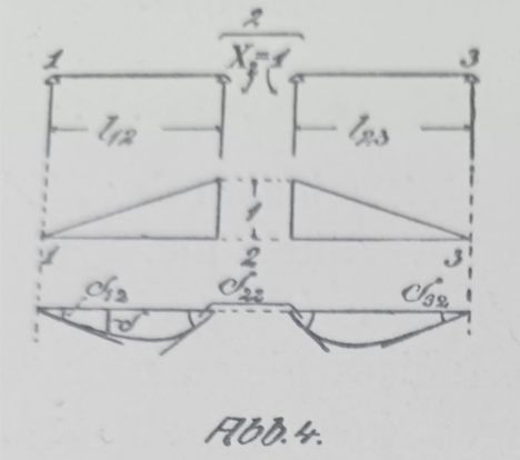
Shear forces
In an unloaded span the shear is constant and equal to (right-hand support moment – left-hand support moment) / span length.
In the loaded span the same expression is used and the simple-beam shear for the unit load is added.
Support reactions
The reaction at any support is the algebraic difference between the shear immediately to the left of the support and the shear immediately to the right.
All of these quantities are therefore available as soon as the number rectangle and the two load terms for the loaded span are known. No further solution of simultaneous equations is required.
5. Extension to multi-leg frames
Rigid joints, column stiffness, fixed or hinged bases, and the small changes required in the rectangle
When the beam is rigidly connected to the columns, the moment immediately to the left of a support is no longer equal to the moment immediately to the right. The difference is taken by the column.
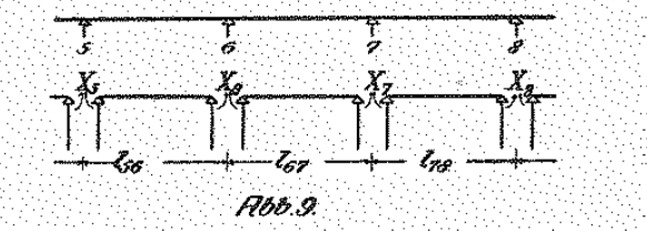
Lewe writes the equilibrium condition at a typical joint as
X – Y = Z [40]
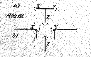
Because the joint is rigid, the three members that meet there (left-hand beam, right-hand beam, and column) must rotate through the same angle.
Because the joint is rigid, the three members that meet there (left-hand beam, right-hand beam, and column) must rotate through the same angle.Lewe first writes the rotations of the two beam ends at a typical support (support 5) under unit moments applied to those ends:
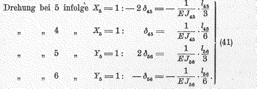
He next gives the rotation that appears at the head of the column when a unit moment Z = 1 acts there. Two cases must be distinguished according to the condition at the foot of the column.
Case 1 – Column base fixed (clamped)

Case 2 – Column base hinged

All three rotations (left beam, right beam and column) are therefore known.
Lewe collects them as formulae (41), (42) and (43).
The requirement that these three rotations must be identical supplies the extra continuity equations at the joint. Lewe writes the pair as


(The same pair is written at every rigid joint.)
When the column flexibilities are substituted into the global system, the coefficient matrix retains the same narrow banded form that appeared for the ordinary continuous beam. The only structural change is that the two diagonals lying immediately beside the main diagonal now carry alternating algebraic signs.
All the earlier machinery remains valid: the continued fractions that produce the end coefficients a11 and ann, the successive ratios i and k, and the filling of the number rectangle by division. The ratios i and k simply pick up the alternating signs. Once the rectangle has been completed, every influence line — beam moments, column moments, shears and reactions — is obtained by the same multiplications that were used for the simple continuous beam.
6. Practical tables and worked examples
What Lewe supplied for the designer and how the numbers are used
Lewe does not stop at the general method. In the second half of the dissertation he works out complete numerical examples so that a designer can see exactly how the number rectangle is built and used.
He begins with a continuous beam that has four intermediate supports (five spans). The spans have different lengths and different moments of inertia.
He first calculates the four flexibility coefficients for each span,

then forms the two continued fractions that give the end coefficients a11 and ann,

records every intermediate ratio i and k, and fills the complete number rectangle by successive division.

Once the rectangle exists, he places unit loads (or uniform loads) in each span in turn and multiplies the appropriate load terms by the rows of the rectangle. The results are the support moments. From those moments he draws the field-moment diagrams, calculates the shears, and finally obtains the support reactions.
The same process is repeated for frames with rigid joints. Lewe supplies ready-made tables of moments for multi-storey frames in which every storey has the same stiffness ratio. The designer simply looks up the coefficient that belongs to the number of storeys and the position of the storey being examined, multiplies by the appropriate load factor, and obtains the beam and column moments directly.

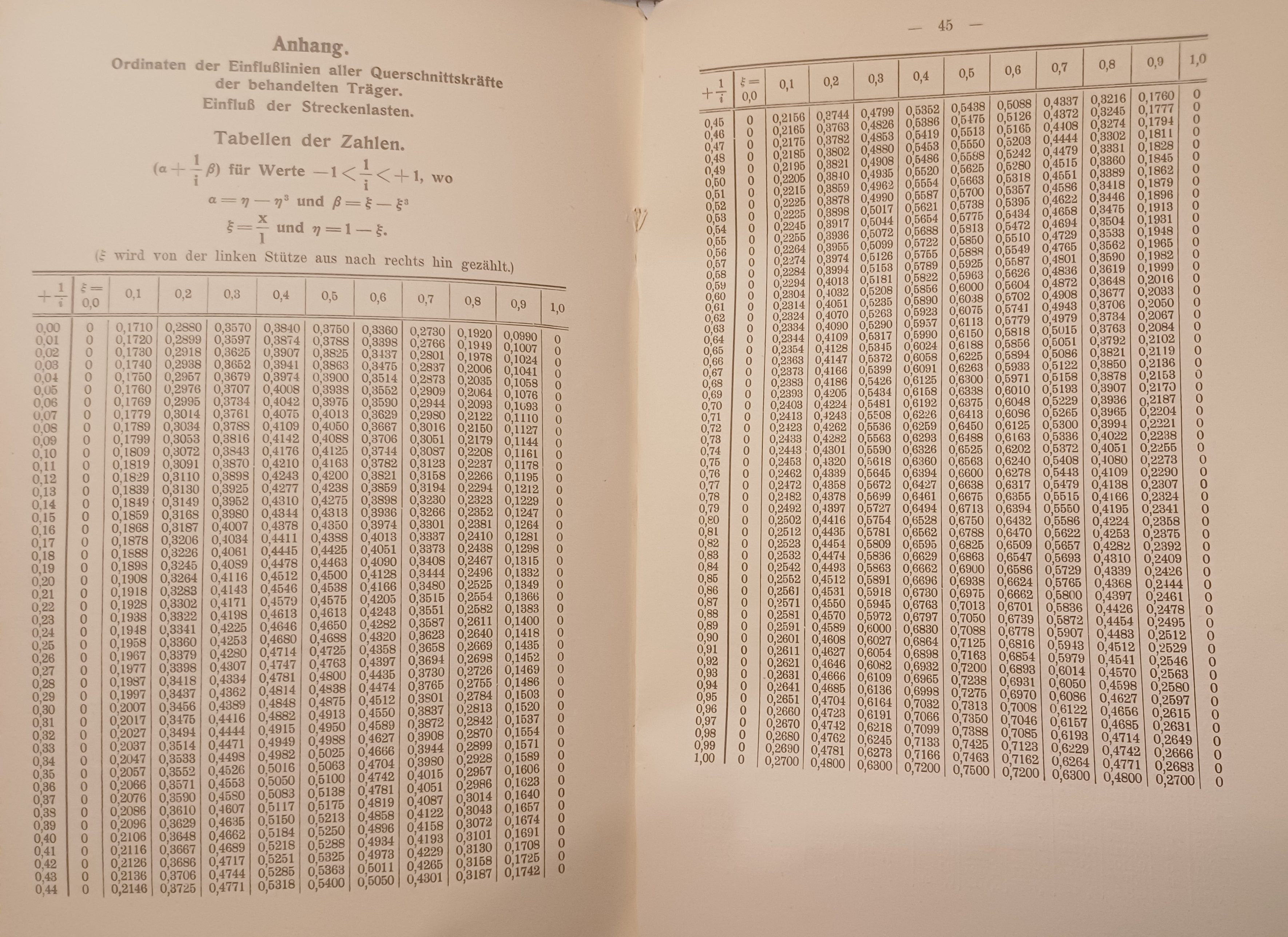
In the appendix he goes one step further and tabulates the actual ordinates of every influence line (moments, shears and reactions) for the beams he has treated. These ordinates are already multiplied by the necessary constants, so the designer can read a number and multiply it by the real load to obtain the force or moment at once.
With the finished tables in front of him, an engineer in 1915 could design a continuous beam or a multi-leg frame without ever having to solve a fresh set of simultaneous equations.
7. Place in the larger history of structural analysis
From Mohr’s elastic line to the matrix methods of the mid-twentieth century
Lewe’s number rectangle sits at a clear point in a longer story.
In the 1860s Otto Mohr gave engineers two lasting tools: a precise graphical construction of the elastic line and a systematic way of writing the three-moment equations that include support settlement. Those contributions turned the continuous beam from a special case into a standard object of calculation.
Graphical statics, developed by Culmann and refined by Ritter, then supplied a visual language for the same equations. Fixed points and force polygons allowed an engineer to trace moments and reactions without writing every algebraic step. Winkler’s tabulated maxima and minima carried the process one stage further by giving ready numbers for the most common equal-span cases.
By 1915 the physical principles were settled and the equations were known. What remained was organisation. Lewe’s continued-fraction evaluation of the banded coefficient matrix, followed by the orderly filling of the number rectangle, converted the existing theory into a compact numerical scheme that could accept unequal spans, variable moments of inertia, and rigid column joints. The rectangle is therefore an early and explicit matrix method, written for hand computation.
The same organisational impulse continued after Lewe. In the 1930s Hardy Cross introduced moment distribution, a successive-approximation technique that again exploited the local character of beam continuity. In the 1950s and 1960s the arrival of digital computers made it practical to assemble and invert large stiffness or flexibility matrices directly. The modern finite-element method is the direct descendant of that line: the structure is divided into simple elements, the element matrices are formed from the same beam or frame flexibilities that appear in Lewe’s work, and the global system is solved by systematic linear algebra.
Lewe did not invent matrix structural analysis, nor did he foresee electronic computers. He did, however, recognise that the banded continuity equations of continuous beams and rigid frames could be reduced to a transparent rectangular array of multipliers. That insight belongs to the same intellectual tradition that later produced the general matrix methods still used today.
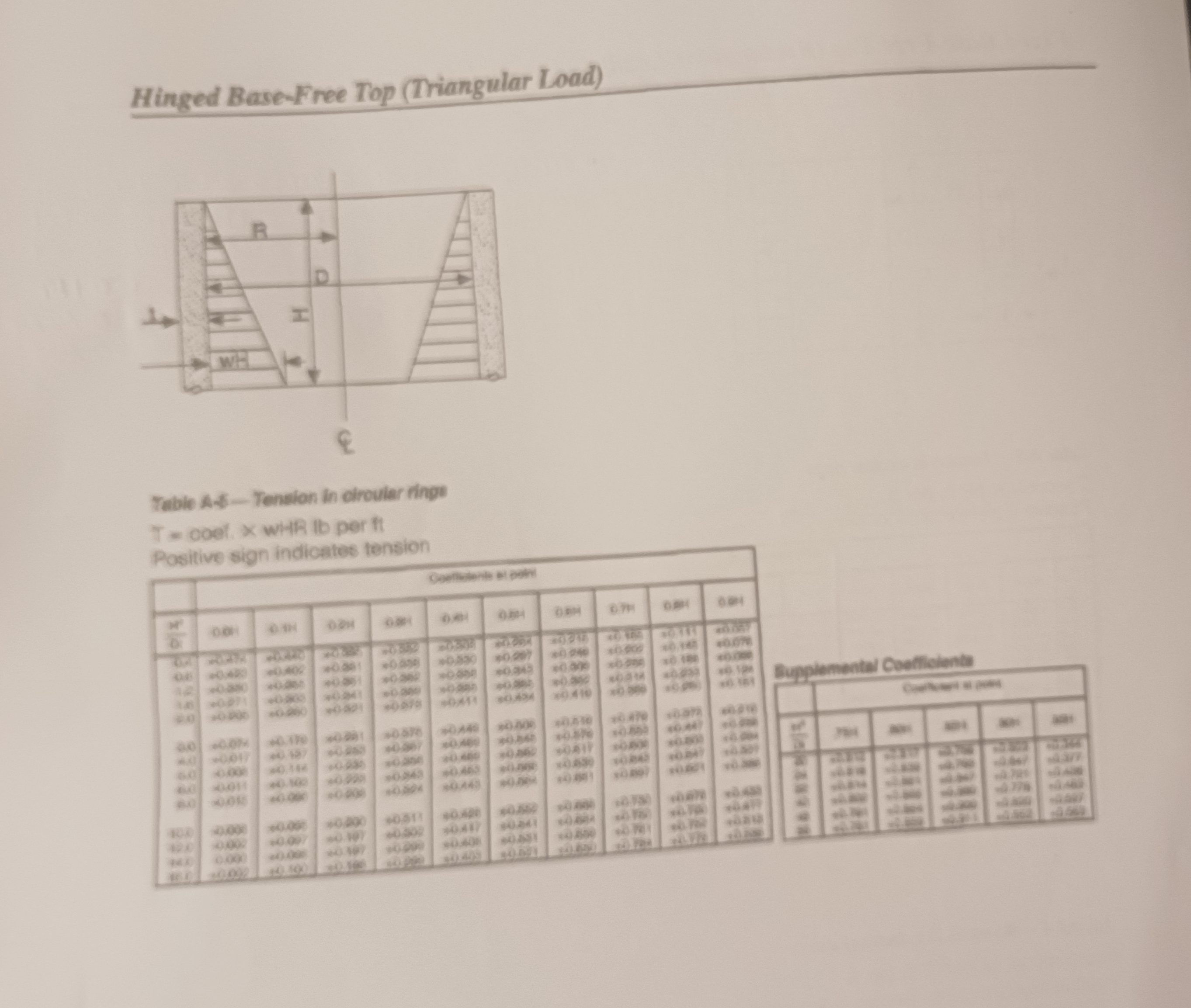
Image from Lewe’s dissertation, compared with Table from Appendices of Domel & Gogate, Circular Concrete Tanks without Prestressing, Portland Cement Association, 1993